What is Time Series Forecasting?

Time Series Forecasting is to try to predict the future based on a sequence of historical events, the historical events are time based that can occur every minute, hourly, daily, weekly, monthly and so on.

Where to start?

The first thing to do is to identify if the data you have is suitable for time series analysis.

Stationary

This is when the mean and variance between data points across the time series are constant and this suggests that there is no trend or seasonality effect that influences the data values. Time series forecasting requires the data to be stationary so that it can be effective and predict accurate results.

Non-stationary

Non-stationary data is when the mean between the data points have different values and the variance between them and across the time frame vary a lot. This indicates that the data is effected by trend and/or seasonality. There are a few tests which can be used to help identify if your data is stationary or non-stationary. Having a unit root in a time series means that there is more than one trend in the series.

How to check if the data is Stationary or Non-stationary?

Visual tests

This is simple test which can be done by first plotting the time series and then checking to see if there is a trend within the plot. The trend could occur at any frequency e.g. weekly, monthly, yearly etc.

Dicker Fuller test

It uses a null-hypothesis to determine whether the data is stationary or not. It checks that your autoregressive model has a unit root, it returns a p-value and if this p-value is less than 0.05 then the null hypothesis can be rejected. In other words, the data is considered as stationary. Test Statistics and p-value are linked and if the test statistic is bigger than Critical Value (10%) it means we can’t reject the hypothesis. The more negative the test statistic, the stronger the evidence for rejecting the null hypothesis of a unit root.

from statsmodels.tsa.stattools import adfuller

def dickey_fuller_test(timeseries):
    #Perform Dickey-Fuller test:
    print 'Results of Dickey-Fuller Test:'
    dftest = adfuller(timeseries, autolag='AIC')
    dfoutput = pd.Series(dftest[0:4], index=['Test Statistic','p-value','#Lags Used','Number of Observations Used'])
    for key,value in dftest[4].items():
        dfoutput['Critical Value (%s)'%key] = value
    print dfoutput

dickey_fuller_test(df_6040_log_moving_avg_diff.iloc[:,0].values)

Results of Dickey-Fuller Test:
Test Statistic                -6.059842e+00     
p-value                        1.220049e-07
#Lags Used                     5.000000e+00
Number of Observations Used    6.800000e+01
Critical Value (5%)           -2.905087e+00
Critical Value (1%)           -3.530399e+00
Critical Value (10%)          -2.590001e+00

The test statistic value should be less than the critical value at 10%, 5% either 1% for the time series to be considered stationary. If it is test statistic < Critical Value (5%) value and > Critical Value (1%), then we can say we are 95% sure that we can reject the null hypothesis.

Decomposition

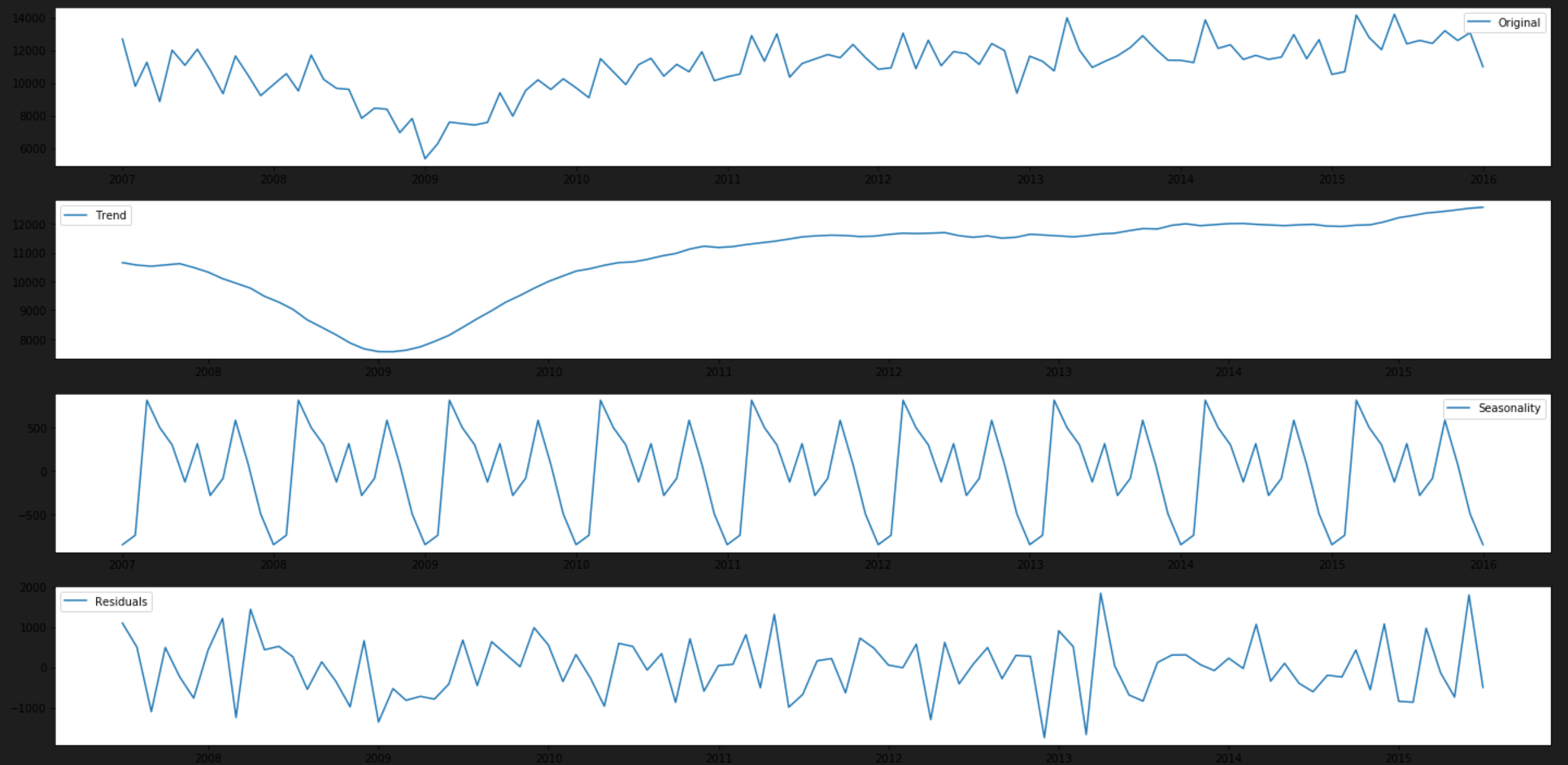
Decomposition is a another process to help determine whether the data is stationary or not. Decomposition deconstructs a time series into several components, each representing one of the underlying categories of patterns such as any trends and seasonality. Once it separates out trends and seansonality from the data the remaining data would be free of trends and seasonality. Not only will you get the seasonality of the data but also the trend and residual.

It uses a number of algorithms to detect and separate out trends and seasonality.

• Step 1 – Remove the Mean
• Step 2 – Calculates a Moving Average
• Step 3 – Calculates the Trend
• Step 4 – Calculates the Cycle
• Step 5 – Calculates the Seasonality
• Step 6 – Calculates the Randomness

from statsmodels.tsa.seasonal import seasonal_decompose

# Using seasonal_decompose() to separate out treads, seasonality and residuals (left over after removing treads and seasonality)
fig, ax = plt.subplots(figsize=(20, 10))
decomposition = seasonal_decompose(df_train_com, model='additive')

trend = decomposition.trend
seasonal = decomposition.seasonal
residual = decomposition.resid

plt.subplot(411)
plt.plot(df_train_com, label='Original')
plt.legend(loc='best')
plt.subplot(412)
plt.plot(trend, label='Trend')
plt.legend(loc='best')
plt.subplot(413)
plt.plot(seasonal,label='Seasonality')
plt.legend(loc='best')
plt.subplot(414)
plt.plot(residual, label='Residuals')
plt.legend(loc='best')
plt.tight_layout()
plt.show()

This will generate a plot with 4 sections, the top containing the original data, then the ‘Trend’, then ‘Seasonality’ and finally the ‘Residual’.

Additive vs Multiplicative

On line 4 of the above code section, there is a parameter called model, there are two possible values for this ‘additive’ and ‘multiplicative’.

The additive model is useful when the seasonal variation is relatively constant over time and the multiplicative model is useful when the seasonal variation increases over time.

Note - that you can use the residual as the dataset for training the model but it is difficult to apply back the trends and seasonality (that we removed) to the forecasted values.

Removing Trends and Seasonality

If our time series is non-stationary, we will need to remove any trends and seasonality effects before creating our model. There are a few ways in which we can do this and I will go through some of them. For some of the forecasting models e.g ARIMA and SARIMA, removing trends/seasonality is not required to perform manually as it is built in part of the model and the model will be able to deal with the trends/seasonality.

Moving Average

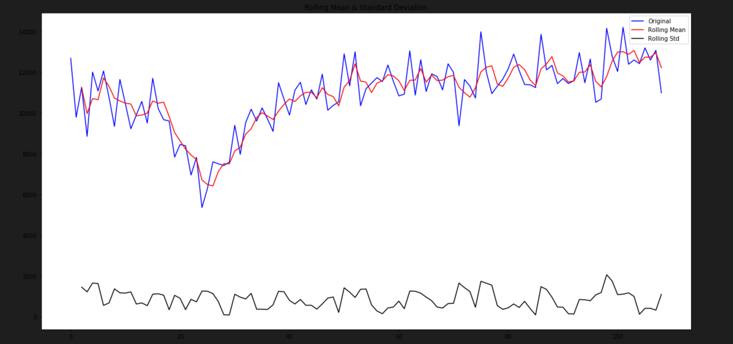
Here we take the average of the values for a rolling time period e.g 12 months and substract this from each of the original values. We then plot the original values along with the rolling mean and rolling standard deviation. Standard deviation (std) is the measure used to quantify the amount of variation between the mean and a data point. The smaller the std means that the data point lies close to the mean.

The difference between the original data point and the mean is used as a potential input of our time series model but first we have to check whether the moving average difference is stationary or not. Time for the Dickey-Fuller test, if we can reject the null hypothesis that would be we can use the moving average difference as input for our model.

fig, ax = plt.subplots(figsize=(20,10))
df.index = df.index.to_timestamp()
plt.plot(df)

moving_avg = pd.rolling_mean(df,12)    # 12 month rolling window
plt.plot(moving_avg, color='red')
display(fig)

df_moving_avg_diff = df - moving_avg
df_moving_avg_diff.head(10)

df_moving_avg_diff.dropna(inplace=True) # The first 12 points wont have a value so removing them

dickey_fuller_test(df_moving_avg_diff.iloc[:,0].values) # Running the Dickey-Fuller test and only passing in the data points and not the time element (date/month/year)

Differencing

Here we adjust the current observation by subtracting the previous observation. There are slightly different methods to deal with trends and seasonality. Differencing can be performed a number of times until the dataset becomes stationary.

Removing Trends

Here you can subtract the previous observation(t-1) from the current observation (t).

new_value = t - (t-1)

Removing Seasonality

Here you can subtract the previous cycle (t-n) from the current cycle (t). Notice, here that we are using ‘n’ instead of 1 as the cycle will be based on your time series intervals and the number of intervals to complete one cycle. For example, if you dataset set contains records on a daily level and the season cycle is one year, then n=365 as there are 365 intervals to complete one cycle.

new_value = t - (t-n)

The ‘t’ doesn’t have to be the actual data value, we can use log of that value. We could use t.log() instead and this can be for both trend and seasonality.

Generate ACF and PACF Plots

ACF - Auto Correlation Function PACF - Partial Auto Correlation Function

These are used to help determine appropriate values for q and p respectively which are then used in model parameters.

ACF - this is a set of correlation coefficients between the time series and lagged versions of itself. This is used to help determine the value for parameter q to be used in MA models.

PACF - this is a partial correlation coefficients between the time series (t) and lagged versions of itself (t_n) but the correlations between them t_n-1, t_n-2, t_n-3 can’t be used to explained the correlation coefficients for t and t_n. This is used to help determine the value for parameter p to be used either in AR, ARMA models

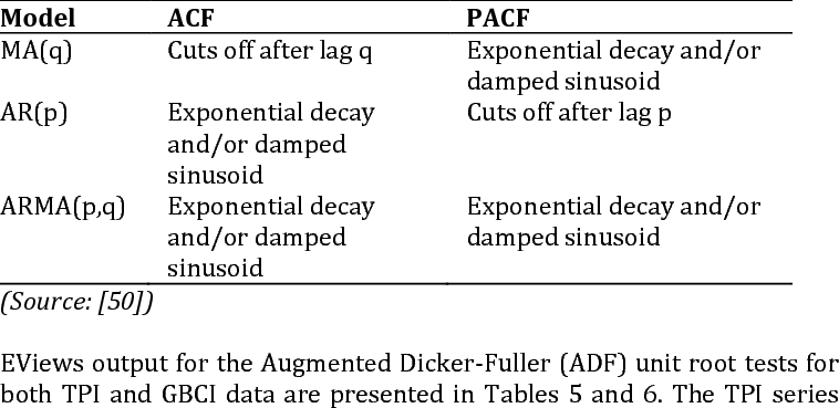
Below is the Behavior of Theoretical ACF and PACF for Stationary Processes

Using the table above, you can identity the most appropriate model to use between AR, MA and ARMA. We can find potential parameter vales for that relevant model from the table as we bascially see whether the ACF or PACF plot slowly decays over time or whether it drops to 0.

Choose a Time Series Model

Next, is to determine which type of model to chose. I will explain a few of them but there are an number of them.

AR - Autoregression, this is where we predict future values based on a linear combination of input values. These input values are past values which is used to predict future values, this is the regression of self.

MA - Moving Average, this uses past forecast errors in a regression-like model. This is different from moving average method to remove trends/seasonality.

ARMA - a (weakly) stationary stochastic process in terms of two polynomials, one for the autoregression (AR) and the second for the moving average (MA). The AR part involves regressing the variable on its own lagged (i.e., past) values. The MA part involves modeling the error term as a linear combination of error terms occurring contemporaneously and at various times in the past.

ARIMA - This is just like ARMA but the ‘I’ stands for intergated which allows differencing to be applied to the data which may be non-stationary. The ‘I’ can be implemented more than once to make the dataset stationary.

SARIMA - Just like ARIMA but the ‘S’ stands for seasonal which allows seasonal differencing.

VAR - Vector Autoregression, this allows multiple features to be part of the model. All the other models mentioned use only one feature the target variable forecasting but VAR allows the target feature plus one or more non-target features for forecasting.

In the next post

We will build a number Time Series models using some of the methods mentioned above.