Stats You Need To Know For Machine Learning

This post will go through some of the required stats you should know for Machine Learning. This will cover many statistical areas but in a brief overview.

Variance and Covariance

Variance is the average of the squared deviation of a random variable from its mean. Basically, it measures how far a set of (random) numbers are spread out from their mean.

Covariance allows us to measure the strength of the association between two variables, if one variable moves in the same directions (up or down) as another then it is said to be a positive covariance. It is said to be negative covariance if the two variables move in different directions.

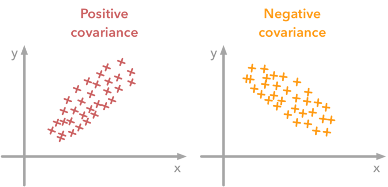source https://www.kdnuggets.com/2018/10/preprocessing-deep-learning-covariance-matrix-image-whitening.html

Standard deviation

Standard deviation (std) is the square root of the variance and this measures how much your data deviates from the mean. A low standard deviation means that the values are close to the mean and high standard deviation shows the values are far away from the mean. In a Gaussian (normal) distribution of data, typically 68% of the data tends to be 1 standard deviation away from the mean in either direction and about 95% of the data tends to be 2 standard deviations away from the mean (again either side of the mean).

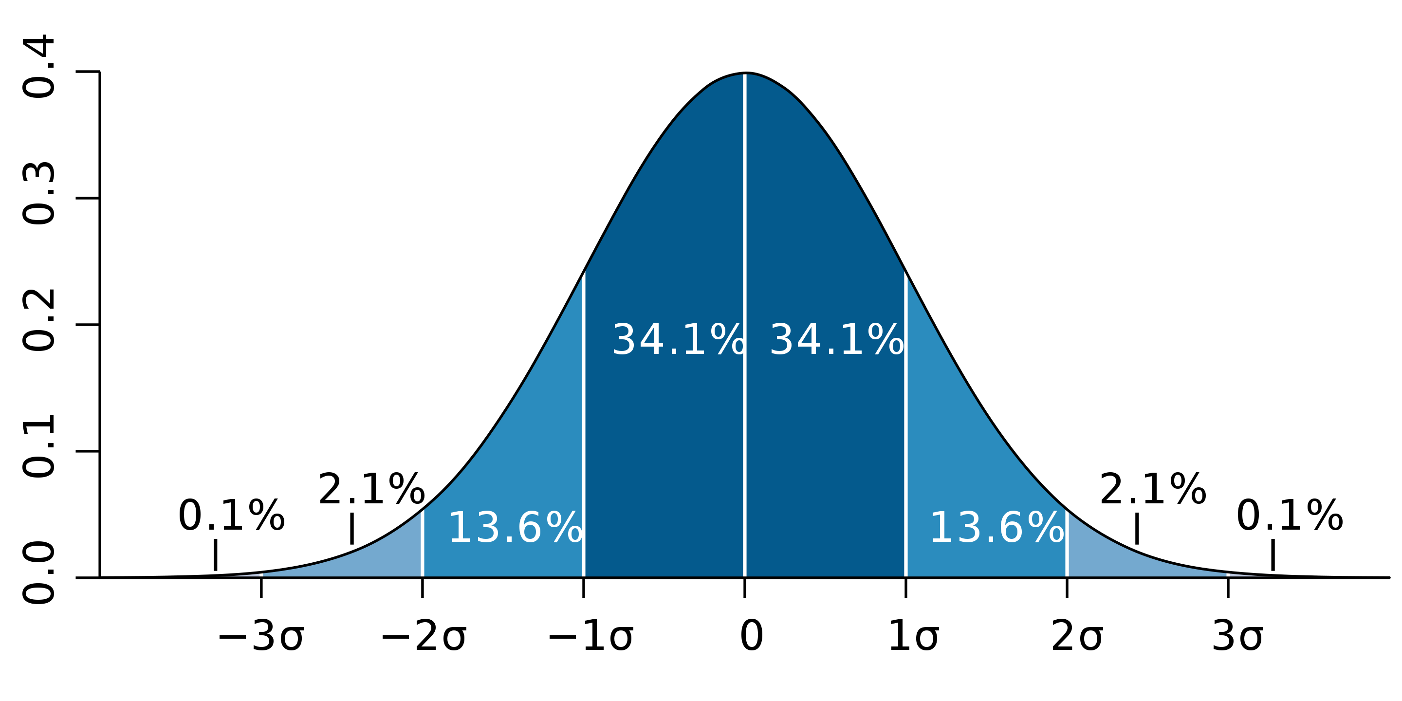source https://en.wikipedia.org/wiki/Standard_deviation#/media/File:Standard_deviation_diagram.svg

Correlation Coefficient

Correlation states the relationship between two variables and the correlation coefficient is a numerical measure of this relationship. The coefficient values is between -1 and 1 where -1 means a strong negative correlation so as one value of a variable goes up, the value of the other variable goes down. 1 means a strong positive correlation so as the values for one variable goes up so does it for the other variable. 0 means there is no correlation at all.

There are 2 main types, Pearson’s and Spearman’s correlation.

Pearson’s correrlation evaluates the linear relationship between two variables where if there is a change in one variable, a constant rate of change is found in the other variable.

Spearman’s correlation evaluates monotonic relationship between two variables where if there is a change in one variable, the change may not always be the same. Spearman’s correlation coefficient is based on ranked values for each variable and not the actual data values.

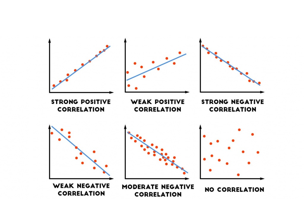source http://danshiebler.com/2017-06-25-metrics/

Central Limit Theorem

This is where means of multiple random samples start to resemble the normal distribution curve more and more as you increase the size of the samples used to calculate the mean. This still applies even if the original distribution of the data is not itself normally distributed. We can use the mean’s normal distribution to create confidence intervals, perform t-tests (see below for information about t-tests) and AVONA (again see below).

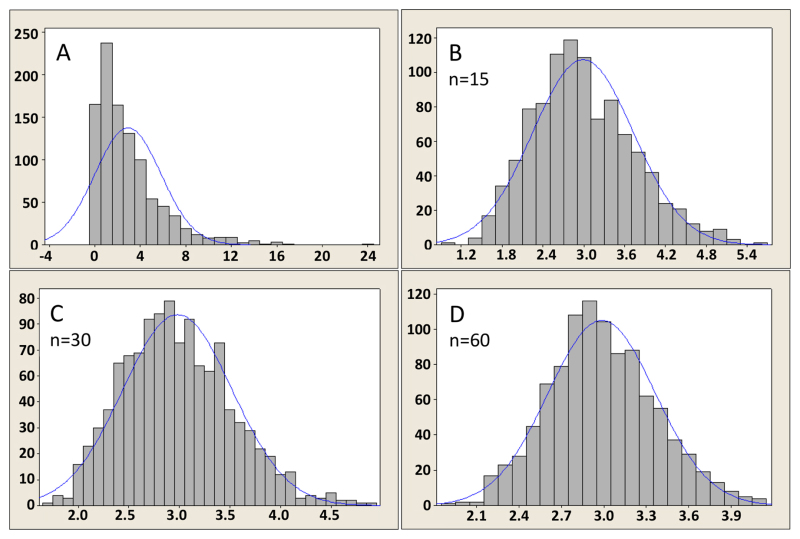source https://www.ncbi.nlm.nih.gov/books/NBK153593/figure/statisticalanalysis_figure7/

Bootstrapping

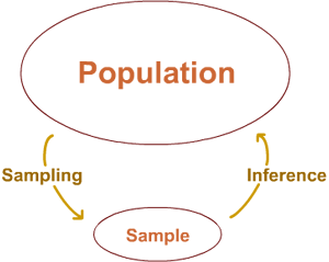
Bootstrapping is a resampling method in which random samples are taken from a dataset with replacement in order to estimate a statistic (e.g. mean, std) for the entire population. Replacement refers to the process that when a data value is selected it is placed back into the data pool to potentially be reselected.

Bootstrapping is a used as a statistical inference method where using the random sampling to infer conclusions about the population.

source https://online.stat.psu.edu/stat414/node/18/

Confidence Intervals

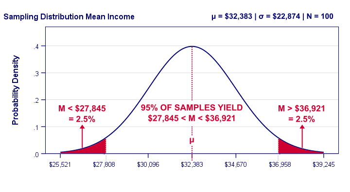
Confidence Intervals uses confidence levels to show a range of where the true value may lie, the most common is 95%. Between the end-points of a 95% confidence interval, it will contain the true value of what we are trying to predict with a probability of 0.95.

source https://www.spss-tutorials.com/confidence-intervals/

Null hypothesis

The hypothesis tests contain a null hypothesis and an alternative hypothesis. The null hypothesis is a general statement that what is observed between two groups is due to chance and nothing special is happening. This is the default assumption by the hypothesis test and it will only be rejected once there is evidence to suggest that the difference is not due to chance.

P-value

The p-value is used to determine whether or not to reject the null hypothesis based on whether it is statistically significant when compared to the significance level usually 0.05.

The p-value is the probability of the sample statistic is at least as bad where the null hypothesis is true.

Z-score, T-test, F-test

Z-score

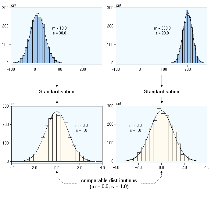
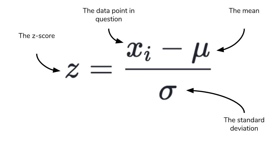
A feature with Gaussian distribution will have a certain unit of measure as its x-axis and the mean and standard deviation of this data will be in that same unit. For example, the distribution of age, the x-axis, mean and the standard deviation will be measured in years. Standardisation ‘converts’ this distribution into a standard normal distribution where the mean is 0 and the standard deviation is 1. The z-score is used to calculate the standard deviation of one value from the mean this is done so that it can be used to easily calculate the probability of an event. It can also be used to compare 2 z-scores/probabilities from two different features even if they have a different unit of measure as they will be standardised.

Z-score is useful large volumes of data.

source http://www.statistics4u.info/fundstat_eng/ee_ztransform.html

source https://www.dataquest.io/blog/basic-statistics-in-python-probability/

T-test

T-tests is a type of inference statistics which compares the values of the mean from two different samples and shows how significant the differences are, it allows us to see if the differences were by chance and something that could not be repeated. In simple terms, it determines whether the samples came from the same distribution of a population. Every t-value has a p-value which is used to indicate the data difference didn’t occur by chance.

We can use this to test the null hypothesis, for example, results from an exam between genders where the null hypothesis is that there will be no difference in the means between genders. We can use a t-test to see if there is difference and if it is very low we can say that the mean samples of the results between genders are different and therefore reject the null hypothesis.

T-test is useful for small volumes of data but a limitation is that the sample dataset must be a good representative of the population dataset and the sample and population is of a normal distribution.

There are 3 types of t-tests:

1. Independent samples t-test which compares mean from two different samples, the difference can be gender, location etc.
   • Null Hypothesis - the mean between the two different samples is equal i.e. there is no difference
   • Alternative Hypothesis - the mean between the two different samples is not equal (NOTE - you can specify whether one is smaller than the other and use one-tailed test)
     
     
2. Paired (Dependant) sample t-test which compares means from two dependant samples with slight variations/conditions such as before and after, two instances. This is a useful test for A/B testing.
   • Null Hypothesis - the mean between the two different variations/conditions is equal i.e. there is no difference
   • Alternative Hypothesis - the mean between the two different variations/conditions is not equal (NOTE - you can specify whether one is smaller than the other and use one-tailed test)
     
     
3. One sample t-test which tests the mean of a single sample against a known mean.
   • Null Hypothesis - the mean of the population will be the same as the mean from a sample dataset of the population
   • We can have two different tests, one-tailed and two-tailed tests which allow for different Alternative Hypotheses
   • Alternative Hypothesis 1 - the sample mean is different when compared to the mean of the population - you would use two-tailed test as it doesn’t matter whether the sample mean is smaller or greater than the population mean, it just has to be different
   • Alternative Hypothesis 2 - the sample mean is either smaller or greater than the population mean - you would use one-tailed test and depending on whether the sample mean is smaller or greater than the population mean you would look at one side of the distribution
     
     

F-test

The F-test uses the f-statistic which is used in ANOVA (see below for more details). It is used to identify if two population variance’s are equal. It does this by comparing the ratio of two variances, this ratio is the F-statistic. So, if the variances are equal, the ratio of the variances will be 1.

The F-statistic is based on the ratio of mean squares, which is simply an estimate of population variance that accounts for the degrees of freedom (DF) used to calculate that estimate.

Anova - analysis of variance

Anova (analysis of variance) is a null hypothesis test to see the statistical significance of means between two or more 0 of data. The null hypothesis is that the means between the groups00 is the same whereas the alternative hypothesis says the means are different. In Anova it can tell you whether there is a significant difference in the means of two or more groups but it doesn’t tell you which ones are different (you can do a post-hoc test to find out which group/s where different). It uses the F-statistic to caluclate the difference and there are two types: One way and Two way Anova.

One way Anova has only one independant variable but many categories to compare for example, the mean of speeding tickets across counties whereas Two way Anova has 2 independant variables, extending the example above another independent variable in addition to counties is gender so we can see if the mean of speeding tickets is different in each county for each gender.

NOTE - the dependent variable needs to be of Gaussian distribution for each group. It can work with non-normal distributions with a small effect on the Type-1 error rate.

Chi-square test

There 2 chi-square tests, one is the goodness of fit test when you have a nominal variable. This checks if a sample data fits the distribution of the population. Basically, it determines if the sample data is a good representative of the acutal population, i.e. the expected results and the actual results are the same/similar. An example is where people might park their cars at night, 70% on the street, 20% in their driveways and 10% in the garage, now we get a sample of data by observing one random street and see if the breakdown of places where people park their cars is similar to our estimate. If acutal percentages is significantly different which would be determined by the p-value then we would reject the null hypothesis that 70% of people park their cars on the street, 20% in their driveways and 10% in the garage.

The other chi-square test is for independence which compares two variables in a contingency table to see if they are related. It tests to see whether the distributions of categorical variables differ from each another so in ensence it see if there is a relationship between two variables. The null hypothesis says that there is no relationship between two categorical variables. The alternative hypothesis is that there is a relationship between the two variables.

Least Squares

Least squares in used in linear regression to ‘draw’ a line of best fit where it tries to minimise the sum of the squared residual values (the distance from a data point to the line of best fit) aka residual sum of squares. This method of minimising the sum of squared residuals is known as least squares regression or ordinary least sqaures (OLS) regression.

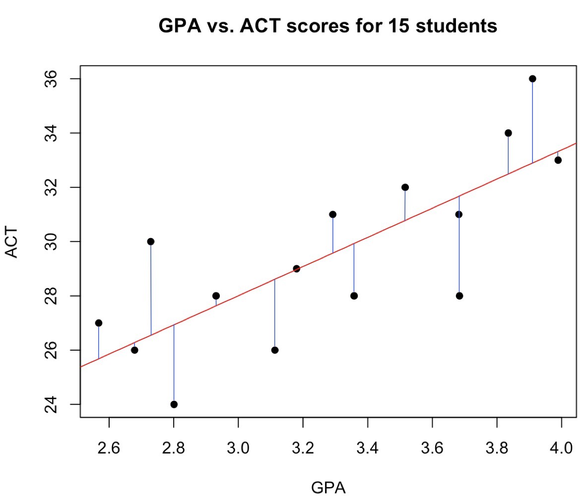source https://towardsdatascience.com/how-least-squares-regression-estimates-are-actually-calculated-662d237a4d7e

K-Fold Cross Validation

Cross validation is a technique to authentic the results of a outcome, its aim is to see how a statistical metric will vary over different fragments of the input data. The idea is that running k-number of validations will help us to see if the model is overfitting and it also helps us to see how the model will perform on different datasets. The idea is to split the all of the data into smaller fragments which is then used to train and then test the model, when one fragment is used to train in another iteration that same fragment of data is used to test the model and every iteration a metric is used to identify the accuracy. The metric is averaged to get an overall accuracy of the model. The k represents the number of interations and fragments to create which tend to vary from 5 to 10.

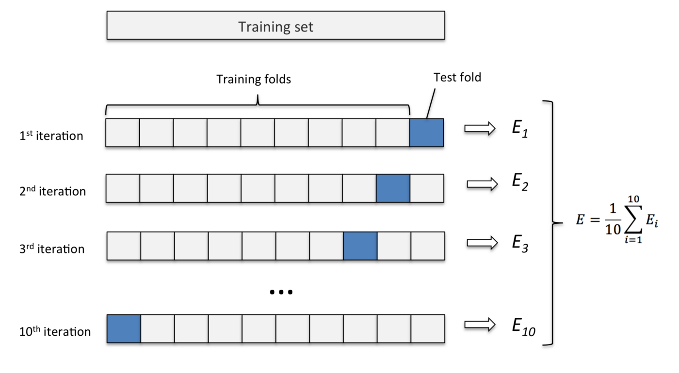source https://medium.com/@sebastiannorena/some-model-tuning-methods-bfef3e6544f0

Precision, Recall and F1 score

To start we need to look at a confusion matrix which shows the number of correctly and incorrectly classed data points. This is typcially used for classification models where we have a positive and negative class. A positive class is something you want to predict e.g. spam email and a negative class is the opposite e.g. no spam, now we need to identify how many data points were correctly predicted as a positive class and negative class but there is the chance that the model incorrectly predicts a data record as positive or negative. We then get 4 types of outcomes:

• True Positive - where the model correctly predicts the positive class
• True Negative - where the model correctly predicts the negative class
• False Positive - where the model incorrectly predicts the positive class i.e. it was actual a negative class
• False Negative - where the model incorrectly predicts the negative class i.e. it was actual a positive class

These outcomes form our confusion matrix.

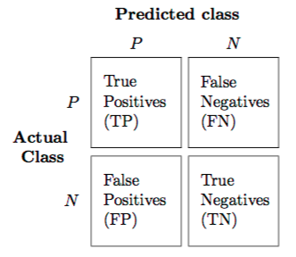source http://rasbt.github.io/mlxtend/user_guide/evaluate/confusion_matrix/

Now we are able to calculate the precision and recall.

Precision tries to answer “What proportion of positive identifications was actually correct?”

Recall tries to answer “What proportion of actual positives was identified correctly?”

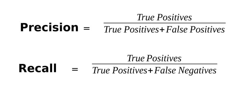source https://medium.com/@raghaviadoni/evaluation-metrics-i-precision-recall-and-f1-score-3ec25e9fb5d3

The F1 score is the weighted average of Precision and Recall which takes both false positives and false negatives into account. F1 is usually more useful than accuracy, especially if you have an uneven class distribution and there is a need to balance. Accuracy works best if false positives and false negatives have similar cost. If the cost of false positives and false negatives are very different, it’s better to look at both Precision and Recall.

source https://medium.com/@raghaviadoni/evaluation-metrics-i-precision-recall-and-f1-score-3ec25e9fb5d3

ROC curve and AUC

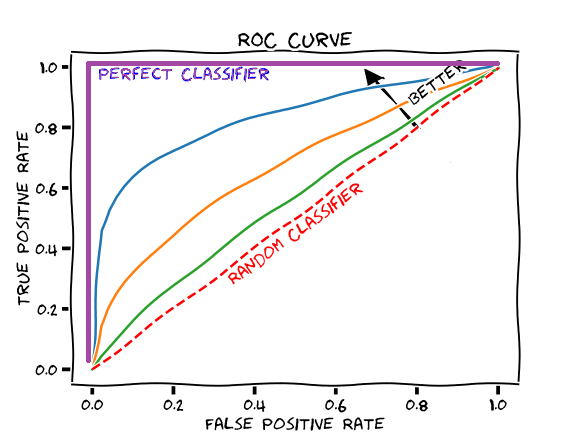
A ROC curve (receiver operating characteristic) curve is a graph which shows how a model performs by plotting the true positive rate (y-axis) and false positive rate (x-axis). It raises the classification threashold which increases the TPR (true positive rate) and FPR (false positive rate) and this is then plotted.

source https://glassboxmedicine.com/2019/02/23/measuring-performance-auc-auroc/

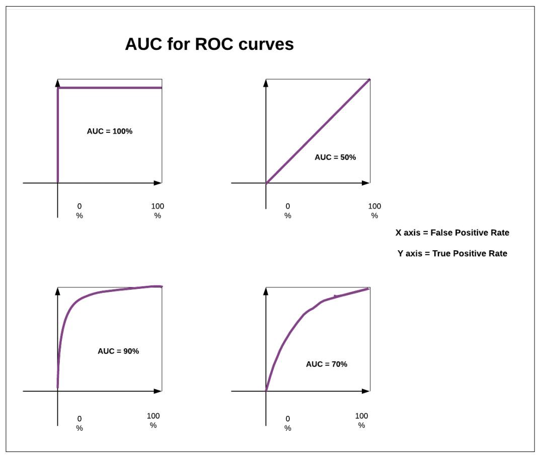
The graph is great but how do we put a number against it? AUC or area under the curve.

AUC is a performance metric we can use to determine how well our model is able to identify positive and negative classes, the area under the graph is calculated to be between 0 and 1 where 1 is the greatest score.

source https://medium.com/acing-ai/what-is-auc-446a71810df9

RMSE

RMSE (root mean square error) is a metric used in regression analysis, it is the average error between the predicted value and actual value.

Expected value

The expected value for a random variable is each possible value the variable can be, multiplied by the probability of that value. The values and the probabilities are summed to produce the expected value.

Eigenvectors and Eigenvalues

Eigenvectors are vectors which don’t change direction and are only scaled when a liner transformation is applied to it. The eigenvalues is the value required to scale the eigen vector. Eigenvectors are used in Principle Component Analysis (PCA) where eigenvectors and their associated eigenvalues are kept.

Entropy, Information Gain & Gini

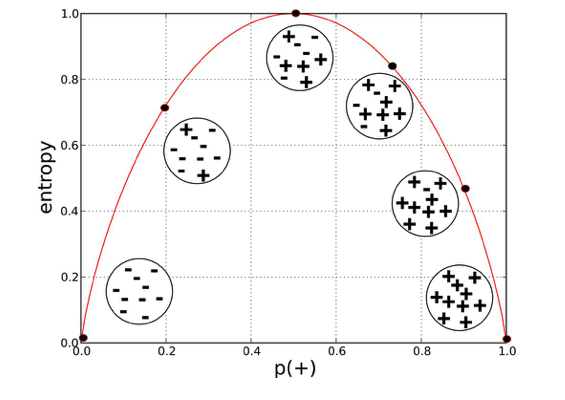
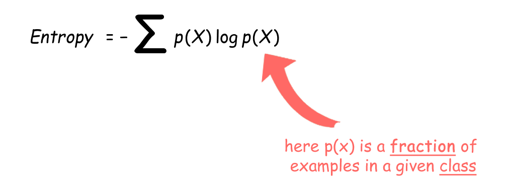
Entropy is a measure of the impurity in data. Entropy is used in Decision Trees to see how good the split is in terms of separating the individual classes. It uses Entropy and Information Gain to judge whether the split of a node in a tree is useful so that records from the same class belong to the same child node. Nodes that have a equal proportion of classes have the maximum Entropy of 1 (this node is heterogeneous) and nodes that only have records with the same class has the minimum Entropy of 0 (this node is homogeneous).

source https://towardsdatascience.com/entropy-how-decision-trees-make-decisions-2946b9c18c8

source https://towardsdatascience.com/entropy-how-decision-trees-make-decisions-2946b9c18c8

Information Gain quantifies the quality of the split, it looks at the Entropy of the parent node and the Entropy of the child nodes after a split. It calculates the change in the amount of impurity removed before and after the split, this value is the Information Gain. The larger the amounf of impurity removed the greater the Information Gain. The Entropy of the child nodes is weighted by the proportion of the number of records in that node and the total number of records across all child nodes for that split.

Information Gain = Entropy of Parent Node - sum(weighted_average% * Entropy of child node) Weighted_average% = Number of records for Child Node A/ Total number of records across all Child Nodes.

A Decision Tree will always select the split that produces the largets Information Gain in a greedy manner as it tries to select the purest splits.

• t is the parent node
• k is the number of child nodes
• n_j is the number of records for child node j
• n_t is the total number of records across all child nodes
• j is a specific child node

Gini is another measure of the impurity in data, it is often used instead of Entropy when building Decision Tree models because Gini doesn’t need to calculate the logs of the values so it is computational faster compared to Entropy.

source https://www.oreilly.com/library/view/mastering-machine-learning/9781788299879/abef109d-e2a4-4c1f-8f54-0e66b17d35f6.xhtml

Cross-Entropy & KL-Divergence

Cross-entropy is a measure of the difference between two probability distributions for a given random variable or set of events. Average number of total bits to required represent event Q instead of P.

KL-Divergence is the average number of extra bits required to represent event Q instead of P.

Normalisation and Standardisation

Normalisation and Standardisation are techniques which allows features of different mangnitudes and units to be represented on the same scale and ‘measured’ in the same units. Every feature has multiple magnitudes which are the individual values for that feature and a unit which is the measurment used to quantify the magnitude e.g. centimeters, miles, kilograms etc. Both of these techniques can be applied to all the numerical features in a dataset and both techniques rescales the data one feature at a time.

Normalisation (aka Min-Max) rescales the data between 0 and 1 and Standardisation rescales the data so that it is of a standard normal distribution where the data has a mean of 0 and standard deviation of 1.

If the original distribution is not Gaussian or the standard deviation is very small, the Normalisation will work better but it is sensitive to outliers. As it

You used normalise/standardise when the algorithms you want to use, uses distance to classify such as k-means, knn, svm or where you use gradient descent in Nerual Networks. It is not useful for tree based models (decision, random forest or boosting trees) as it won’t make a difference where the data is scaled or not as it makes the split based on a criterion.

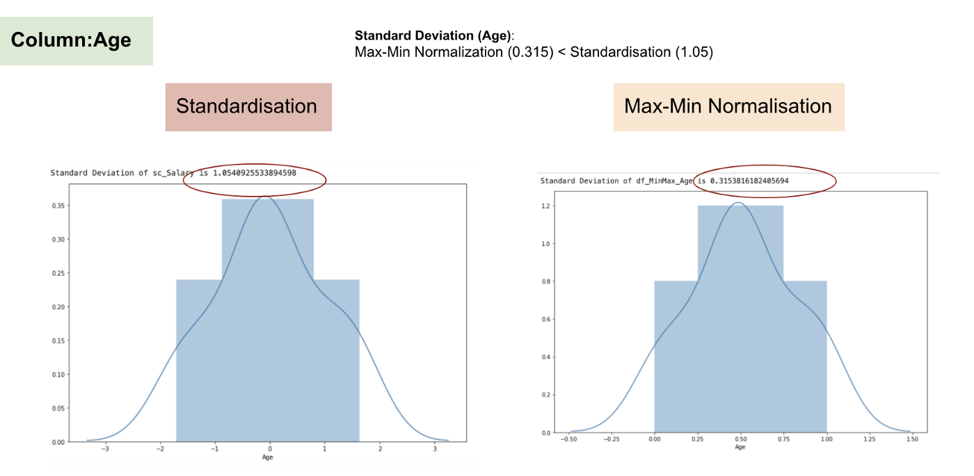source https://www.kdnuggets.com/2020/04/data-transformation-standardization-normalization.html